Dynamiqs, Put to Work

Following unitaryHACK26, the team at Alice & Bob breaks down their open-source work on Dynamiqs in this guest contribution. Thank you to Nicolas Lepage, Ronan Gautier, Adrien Bocquet, and Matthieu Patrizio for serving as maintainers, and to Laurent Prost and the team for their support of the hackathon.

Unitary Foundation runs unitaryHACK every year, a hackathon built around real issues from open source libraries. This year, Alice & Bob submitted five issues from Dynamiqs, and contributors picked up every one of them.

The five range widely, but converge on the same thing: a library that’s reliable under load, easy to work with, trustworthy, and performant enough to build chips with. A new test suite for the stochastic solvers (#1079) validates a tool that gets used daily. Work on the QArray manipulation utilities (#1080, still in progress) is smoothing out small frictions in daily use. Broader type coverage across the codebase (#1081) makes the library production grade, easier to maintsain and to build on. Native Hessian computation (#1082, also merged) enables the use of advanced optimisation tools. And a large benchmark suite (#1083, in the works) will allow us to know exactly the performance and accuracy of the library.

Thanks to spital, Ronit-Raj9, and Mayank447 for getting their pull requests merged, and to JAMA4666 and jackson5689 for their work on the two still in progress.

Building a quantum chip takes more than analytical formulas. As real devices grow in complexity, simulation becomes the only way to move fast — testing and optimising designs before fabrication, then characterising and calibrating the real chip through a digital twin after. You cannot fabricate every variant and measure it, so you simulate. And the simulations that matter are not textbook two-level toy models. They are open quantum systems with many modes, large Hilbert spaces, and dynamics that span wildly different timescales.

Dynamiqs was built for that regime, and for nearly any open quantum system, not only cat qubits. It is the engine we reach for when a question has to be answered at full scale rather than approximated down to something convenient. Below we put it to work on two problems drawn from cat-qubit design, chosen for their large Hilbert spaces and stiff dynamics, and show that one library carries both within a single shell.

Dynamiqs in a nutshell

Dynamiqs is a simulation tool that solves the differential equations of quantum time-dynamics: the Schrödinger equation, the Lindblad master equation, and their stochastic cousins. Built on JAX with a deliberately small, focused API, it gives you:

• CPU and GPU support. Write the simulation once, run it on GPU with a single call. For large systems, this can give significant speedups.
• Batching. Sweep over Hamiltonians, initial states, or any parameter by passing a list instead of a single input. These simulations get optimally run in parallel.
• Differentiability. Every solver is differentiable, so gradients of any output with respect to any parameter come straight from JAX, the engine behind optimal control and parameter fitting.
• The full solver family. Closed systems (sesolve), open systems (mesolve), and trajectory-level stochastic solvers (dssesolve / dsmesolve) for continuously measured systems.

Our companion post walks through the API and design philosophy in more detail (read it here). Here we want to highlight two choices that show Dynamiqs was built specifically to solve the Lindblad master equation well.

A custom sparse format. Quantum optics operators (annihilation, creation, number, and their products) are banded — almost every entry is zero, and the non-zeros sit on a handful of diagonals. Dynamiqs stores operators in exactly this shape, as a sparse diagonal (DIA) format, keeping only the populated diagonals, which lowers memory and compute cost, and maps cleanly onto GPU hardware.

Solvers that respect physics. Dynamiqs integrates Rouchon methods designed specifically for the Lindblad master equation, rather than generic ODE solvers retrofitted to a quantum problem. A valid density matrix must stay positive semidefinite and trace-one (its evolution must be completely positive and trace-preserving), and generic integrators quietly drift away from that. Rouchon solvers strictly preserve those properties.

A focused library with good defaults beats a sprawling one, and unitaryHACK helped us keep it that way, expanding type coverage across the codebase (#1081) and filling out the QArray manipulation utilities (#1080).

Now let’s put it to work. Nothing below is cat-specific: the solvers, the sparse format, and the batching all apply the same way to any bosonic or spin system. We will walk through two problems, each chosen to showcase the maturity of the library: one running the forward simulation at full scale, and one running it backwards to recover a model from data.

Sixteen CNOTs at once

Our first problem is a CNOT gate between two dissipative cat qubits, a flagship operation for cat-qubit architectures and a deliberately heavy simulation.

Why it’s hard. The system has three bosonic modes: a control cat, a target cat, and a buffer mode that drains entropy away. With comfortable truncations (24 × 8 × 24), the Hilbert space is 4,608-dimensional, so each density matrix is a 4,608 × 4,608 object. The quantum system is governed by the Lindblad equation.

$$\dot\rho = -i[H,\rho] + \sum_k \left( L_k \rho L_k^\dagger - \tfrac{1}{2}\{L_k^\dagger L_k, \rho\}\right)\\ H = g_2 (a_c^2 - \alpha_c^2) b_c^\dagger + \mathrm{h.c.} + g_{cnot} (a_c + a_c^\dagger) (a_t^\dagger a_t - \alpha_t^2) \qquad L = \sqrt{\kappa_b} \hat b_c .$$

The first term, together with the strong buffer loss $L$, autonomously stabilises the control cat through two-photon exchange (this is the “Zeno” mechanism). The second term rotates the target conditioned on the control (the CNOT itself) over a gate time $T = \pi/(4\alpha_cg_\mathrm{cnot}) \approx 300\ \mathrm{ns}$.

It is also genuinely stiff. Engineered dissipation (the fast buffer damping, $\kappa_b/2\pi = 10$ MHz) and the Hamiltonian’s non-linearity in $\hat a$ (operator products above second order, like $g_2\,\hat a_c^2\,\hat b_c^\dagger$) make the problem stiff, and it must be solved over the comparatively long run time of the gate ($g_\mathrm{cnot}/2\pi \approx 0.2$ MHz). An adaptive integrator resolves that fast dynamics across the long gate, so a single run costs many thousands of time steps.

Running all sixteen at once. To characterize a gate you don’t run it once, you run quantum process tomography: sixteen input states, the products of the four cardinal logical states $\{\ket0, \ket+, \ket{+i}, \ket1 \}$ on each of the two cat qubits. In Dynamiqs that is not sixteen scripts in a loop. You stack the sixteen 4,608-dimensional inputs and hand them to mesolve as a batch:

import jax.numpy as jnp
import dynamiqs as dq

alpha = 2.0
n = 32  # Hilbert space dimension per mode

cardinal_states = [
    dq.coherent(n, alpha),                    # |0>
    dq.cat(n, alpha, 0),                      # |+>
    dq.cat(n, alpha, jnp.pi / 2),             # |+i>
    dq.coherent(n, -alpha),                   # |1>
]

rho0_batch = [
    rho_c & rho_t & dq.vacuum(n)
    for rho_c in cardinal_states
    for rho_t in cardinal_states
]

result = dq.mesolve(H, [L], rho0_batch, tsave)  # 16 states simulated at once

Three of the library’s bets compound here. The sparse format reduces the memory and compute cost of every operator by roughly a factor of the problem size, which at CNOT scale pays off spectacularly. Batching turns sixteen sequential solves into one large one. And we lean heavily on GPU acceleration to handle the dense density-matrix operations that dominate the right-hand side. On an H100 GPU the batch runs in a few seconds, fast enough to fold tomography into vast parameter sweeps and optimisation loops.

Figure 1 — A 4 × 4 grid of Wigner functions, one panel per tomography input (rows: control preparation; columns: target preparation), animated across the gate. We trace out the buffer and show the target mode, because that is where the action is visible.

Why you’d care. This is the inner loop of any multi-mode gate design, cat qubits included: change a parameter, re-run the tomography, read the fidelity. Doing all sixteen states at once, on a stiff multi-mode system, in seconds rather than minutes, is what turns an overnight sweep into an interactive afternoon.

Reverse-engineering a chip from its noise

In the digital twin context, simulation is not only a validation tool but an optimisation tool, used for characterisation: knowing our chip’s true parameters removes the uncertainty inherited from fabrication. Demonstrating this requires a validation problem where the ground truth is known. We start from a known system, use simulation to generate noisy, experiment-like data, and then show that fitting this emulated data recovers the system’s true dynamics, all done in Dynamiqs.

Step 1: Emulate a realistic experiment. Our known system is a two-mode model, a memory mode and a readout mode, given the messy reality of a real chip: Kerr and cross-Kerr terms, detunings, and delayed control pulses. We run the diffusive stochastic Schrödinger solver, dssesolve, to emulate what a lab would actually record, trajectory by trajectory. Averaging over thousands of trajectories and folding in a finite measurement efficiency turns this into a complex voltage, our noisy experiment-like data, shot noise included. These records are only trustworthy because the stochastic solvers behind them are validated. unitaryHACK contributors hardened exactly that corner, adding a test suite for the stochastic solvers (#1079).

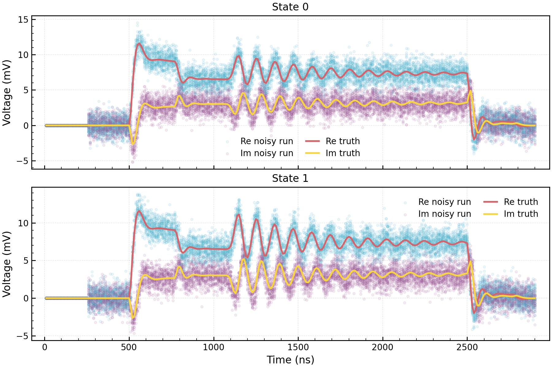
Figure 2. A synthetic measurement dataset, one panel per initial state. Blue and teal points are the noisy real and imaginary readout quadratures (averaged over many trajectories), and the red and purple dashed lines are the ground-truth voltages behind them.

Step 2: Inverse problem. Now, to validate the characterisation process, we pretend we have forgotten the 16 parameters and treat them as unknowns. We predict the voltage with the deterministic, differentiable master-equation solver, compare it against the noisy data, compute a fully differentiable loss, and descend.

What makes this loop practical is automatic differentiation. Dynamiqs computes the gradient of the predicted voltage with respect to every parameter natively and at low cost, straight from the forward pass. That lets us use efficient steepest-descent algorithms directly, instead of falling back on expensive and lower accuracy finite-difference estimates or derivative-free methods.

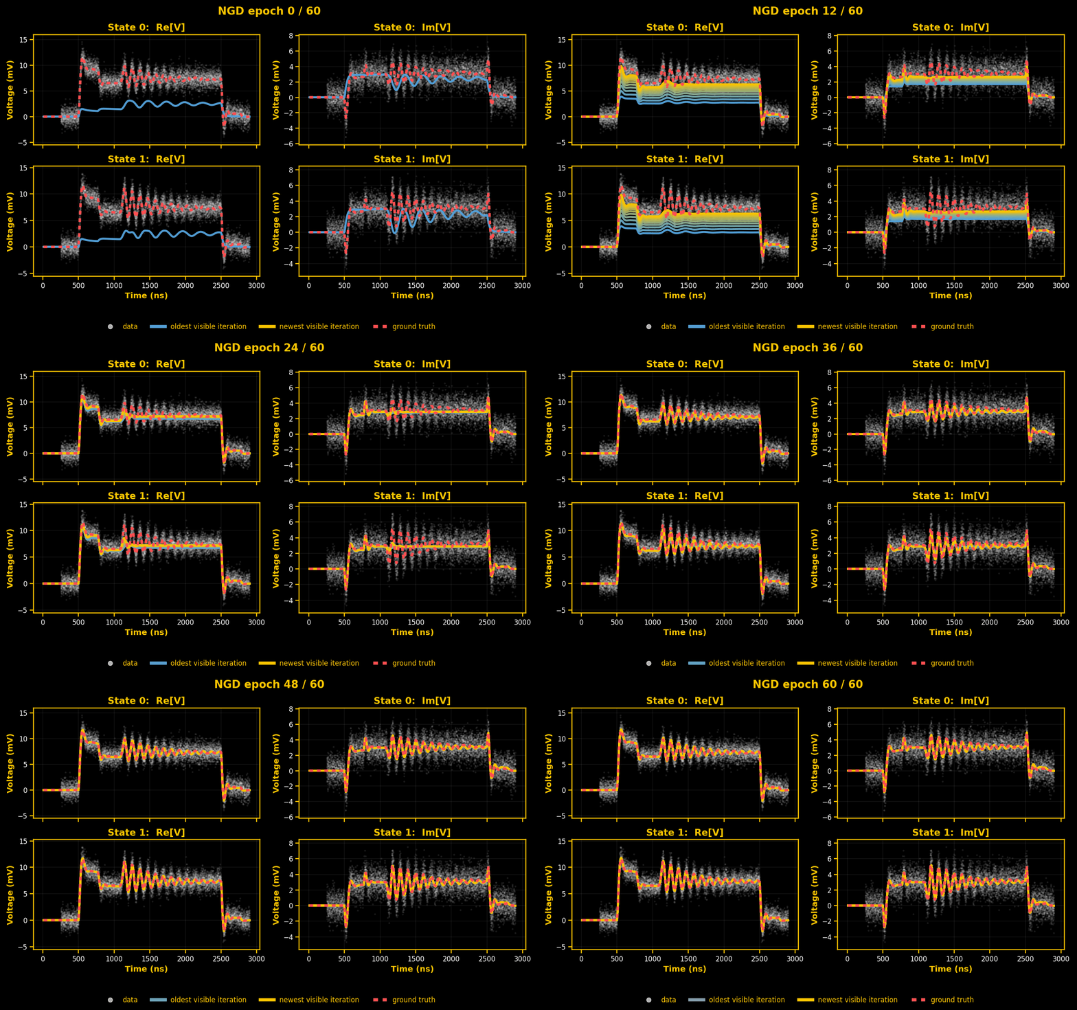
Figure 3. The natural-gradient fit converging over 60 epochs. Rows are the two initial states, columns the real and imaginary quadratures. Grey points are the noisy data, red dashed is the ground truth, and the solid curve (blue early, yellow late) is the running prediction.

Why you’d care. This is device characterisation, learning the true properties of a chip from its measurements, done as a closed, fully differentiable loop. Knowing the model exactly means you know what your system really is, which enhances the accuracy of the predictions. The same two ingredients that make Dynamiqs fast on the forward problem (stochastic solvers for realistic records, differentiability for the inverse problem) turn out to be exactly what calibration and characterisation need. And it is about to get faster: new Hessian support through the solvers, landed during unitaryHACK (#1082), opens the door to Newton’s method and even faster convergence.

The road ahead

Working through problems like these taught us something concrete about our own engine. Pushing toward ever larger simulations, and eventually toward running thousands of them at once, has made one thing clear: we are using GPUs outside the context they were designed for. GPUs are built for dense matrix multiplication, and quantum simulation asks something different of them. That is a good problem to have, because it tells us exactly where to push:

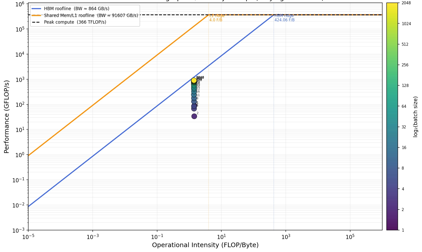
Figure 4. Roofline analysis of a Step 2-scale simulation across batch sizes (1 to 2048). Each point plots performance against operational intensity; the blue line is the HBM bandwidth ceiling, dashed is peak compute. Batching adds FLOPs without changing intensity, so points climb straight up and saturate against the HBM roofline, the signature of a memory-bandwidth-bound problem.

• A minimal-movement sparse @ dense kernel. The dominant cost in the master-equation right-hand side is multiplying a sparse operator into a dense state. We’re rewriting that kernel to touch each byte of the state as few times as possible.
• Pushing the stochastic solvers. Trajectory solvers are vectorial and embarrassingly parallel (thousands of independent trajectories), so their compute-and-memory profile differs from the deterministic solvers and wants its own optimisation.
• A steady-state solver suite. Many questions don’t need the trajectory at all, only where it ends up. Dedicated steady-state solvers will answer those directly.

To steer all of this we need to measure it, which is why a standardized benchmark suite came out of unitaryHACK as well (#1083).

Come build with us!

Dynamiqs is open-source and we mean it. Whether you want to simulate a gate, characterize a chip, or optimise a control pulse, the library is pip install dynamiqs away.

Huge thanks to everyone who contributed during unitaryHACK.

Explore the docs at dynamiqs.org, dive into the source on GitHub, and open an issue or a pull request. Let’s push the performance of quantum simulation, together.